
ARmask - HMI Active Region Full-Disk Masks
Overview
This is a full-disk data product that currently identifies magnetically active pixels. The corresponding data product is hmi.Marmask_720s. There is a corresponding near-real-time data product, which is used to get timely space weather information, called hmi.Marmask_720s_nrt.
The mask is an integer (char, or BITPIX = 8) value at each pixel. Currently the integer can be one of three values: 0 for off-disk, 1 for quiet, and 2 for magnetically active. We hope to add a facula class, especially as the intensity images become more well-calibrated.
We use two image series, magnetograms (from hmi.M_720s) and intensitygrams (from hmi.Ic_720s), to determine class membership. This first iteration of the masks concentrates on active regions, so we rely on the magnetograms almost exclusively to compute the masks. The mask image is computed and stored in "focal plane" or image coordinates, so mask values at a given (i,j) pixel correspond with magnetic activity at that (i,j) pixel.
Methodology
The methods used were developed by Turmon, Pap, and Mukhtar (), and subsequently refined to allow for spherical geometry (). The basic idea is that the mask should optimize a function containing two terms, one for pixel-by-pixel agreement of the observed (M,Ic) values to what is expected for a given class, and another for smoothness across adjacent pixels. The first term, which matches observed (M,Ic) values to the expected scatter for each class, is dominant in the calculation. The smoothness term only affects mask values that are near the boundary between classes (i.e., have an (M,Ic) value that is inconclusive). Geometrical information is encoded in the smoothness term.
The overall effect does not correspond to a threshold rule on M and Ic. Boundaries between classes follow non-axis-parallel contours that are a property of the competition between the expected scatter of the two classes.
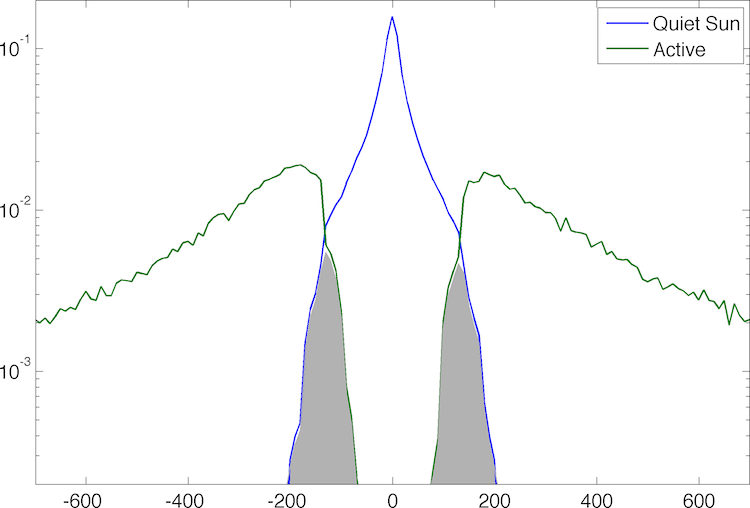
As noted above, the current processing uses the magnetogram almost exclusively. The plot below shows the distribution of quiet Sun pixels (blue line) and magnetically active pixels (green line) versus magnetic field (x axis, in HMI Gauss). The gray areas are pixels whose classification can be changed if the spatial cues in the objective function indicate that it would be beneficial enough.
[http://sun.stanford.edu/~turmon/jsoc-wiki/classhist2-2011-feb-14-small.png]
The method is implemented in a pipeline module called hmi_segment_module. It requires about 40 seconds per 4096x4096 image.
Example Images
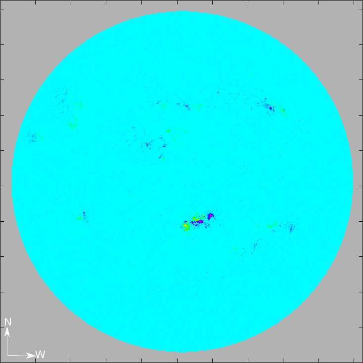
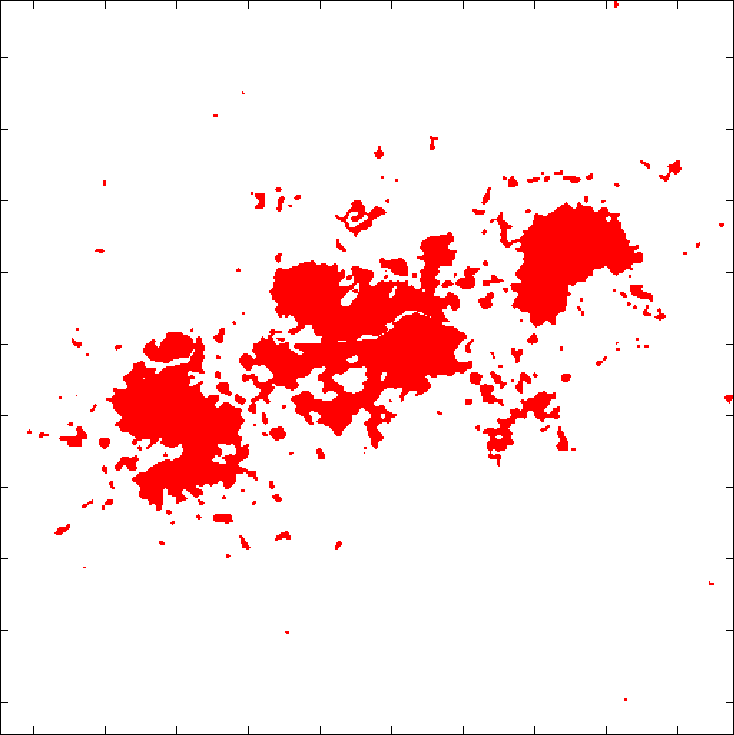
This is a labeling and the corresponding magnetogram from 2011 February 14.
[http://sun.stanford.edu/~turmon/jsoc-wiki/mask2011-02-14.png] [http://sun.stanford.edu/~turmon/jsoc-wiki/mag2011-02-14.png]
This is a detail from the same mask image. It shows the structure at fine spatial scales.
[http://sun.stanford.edu/~turmon/jsoc-wiki/mask2011-02-14-zoom.png]