
|
Size: 2263
Comment:
|
Size: 8690
Comment:
|
| Deletions are marked like this. | Additions are marked like this. |
| Line 3: | Line 3: |
=== Note === This data product was released in April, 2012. |
|
| Line 7: | Line 11: |
| is a coherent magnetic structure at the scale of a solar active region identified in one or more HMI line-of-sight magnetograms. HARPs are typically observed over an extended time interval (e.g., days), and tracked from one image to the next. | is a coherent magnetic structure at the scale of a solar active region initially identified in a sequence of HMI line-of-sight magnetograms. HARPs are typically observed over several days (possibly as long as a disk passage), and tracked from one image to the next. At each time, the HARP bounding box and a mask that encloses the HARP are recorded. |
| Line 9: | Line 15: |
| The HARPs in the data series `hmi.MHARP_720s`, which is indexed by an integer identifier, `HARPNUM`, and by `T_REC`. The HARP will often be linked with a NOAA Active Region. This data series provides pointers to information covering the entire disk passage for each HARP in the HMI catalog, as well as summary information such as per-region integrated flux, for each `HARPNUM` at each `T_REC`. | The HARPs are in the data series `hmi.Mharp_720s`, which is indexed by two prime keys, an integer identifier, `HARPNUM`, and the time, `T_REC`. A particular `HARPNUM` will often be linked with a NOAA Active Region (see the appropriate keywords, e.g. NOAA_AR, NOAA_NUM, NOAA_ARS). This data series provides pointers to information covering the entire disk passage for each HARP in the HMI catalog, as well as summary information (e.g., integrated flux over the HARP), for each `HARPNUM` at each `T_REC`. Because we use 720s HMI data, some HARPs contain as many as 1500 distinct `T_REC`'s, and some as few as three. Besides the keywords mentioned above, the HARP data series contains one 2D data segment, `BITMAP`, which is a mask image of the extent of the HARP at a given time. |
| Line 11: | Line 21: |
| The data series tracks patches by associating information from other data series using links to maps and parameters computed for patches identified in individual magnetograms and intensity images. There are no actual data segments, just links to vector, line-of-sight, and intensity data and associated keywords. | The HARPs are found by analyzing the active region masks in `hmi.Marmask_720s`. (The masks are in turn derived from `hmi.M_720s` and corresponding intensitygrams, `hmi.Ic_noLimbDark_720s`.) All three of these data products are full-disk images, in helioprojective-tangent coordinates (that is, as projected on the focal plane, and not remapped to a latitude-longitude system). The `BITMAP` segment of the HARP data series indicates exactly which pixels in the 720s magnetogram are part of the HARP. It is a rectangular cutout from the full-disk images referred to above, typically several hundred pixels in each dimension, with special values indicating whether a pixel is on-HARP or not. |
| Line 13: | Line 28: |
| === HARP Data Series Keywords === | The data series can be used by following the links to associated vector, line-of-sight, and intensity data. For diagnostic or summary purposes, plots of individual keywords, such as integrated flux or size of the HARP, are also useful. |
| Line 15: | Line 31: |
| # SERIES INFO . DATANAME = HARP . RETENTION = 0 . ARCHIVE = 0 . PRIMEKEYS = HARP_ID, T_REC |
== Methodology == |
| Line 21: | Line 33: |
| # PRIME KEY INFO . HARPID, INT . T_REC, TIME, Slotted . T_REC_STEP = 12MIN . T_REC_EPOCH = 1976.12.31_23:59:45.000_UTC |
Once localized sites that are magnetically active have been found (i.e., building on the full-disk active region masks) the HARP identification problem consists of two pieces: spatially grouping magnetic activity into objects on the scale of active regions, and tracking these objects from image to image. The grouping problem is harder, because flux emergence can cause formerly isolated ARs to merge. This means that a given HARP cannot be declared complete until it has disappeared in view of the observer, or rotated off the visible disk. Consequently, final HARPs are delayed by about a month. |
| Line 27: | Line 35: |
| # PATCH INFO . PNUM, link, "PNUM", patch - '' The patch number of the HARP at T_REC in the Patches_Found dataseries'' . AREA, link,"AREA", patch - '' The AREA keyword of the patch`` . I_MIN, link, "I_MIN", patch . FLUX, link,"FLUX",vecpatch - '' The computed flux of the vector field in the patch '' . BTOT, link, "BTOT", vecpatch . # OTHER information about the patches |
It is important to track HARPs up to the limb, so that all the history of the HARP can be taken in to account in making grouping decisions. Consequently, the grouping criterion takes the spherical geometry into account. |
| Line 35: | Line 37: |
| # SEGMENT INFO - links . data: arp_map, link, patch - '' Pointer to the bitmap of the patch '' . data: blos, link, patch - '' Pointer to pointer to line-of-sight magnetic field data '' . data: BTOT, link, vecpatch - '' Pointer to pointer to vector magnetic field data '' |
We expect it will be useful to have easy access to the precursors and successors of the HARP. So, we extrapolate the area containing the HARP backwards in time from where it was first detected, and forward from the time where it vanished, two days in each direction. (Or less, if the entire region would rotate off-disk in this time.) This has the effect of expanding the range of T_REC associated with each HARP. |
| Line 40: | Line 41: |
| # LINKS . link: patch, "Patches_Found", static ''(because PNUM is arbitrary) '' . link: vecpatch, "Vector_Patches", dynamic |
The HARP identification component consists of two parts, a grouping/tracking component, implemented in Matlab, and a data ingestion component, implemented as a JSOC module. |
| Line 44: | Line 43: |
| === Related Data Series === . PatchesFound |
== HARP Feature Scale == The following images show how the convolution kernel used for spatial grouping of active regions compares to a small active region at disk center. The units on the top two plots are HMI pixels. The bottom plot shows the convolution kernel at the same scale. [http://sun.stanford.edu/~turmon/jsoc-wiki/kernel-scale-ar-mag-small.png] [http://sun.stanford.edu/~turmon/jsoc-wiki/kernel-scale-ar-mask-small.png] ||<25%> [http://sun.stanford.edu/~turmon/jsoc-wiki/ar-grouping-kernel-center-small.png] ||<15%> When at the limb, the convolution kernel is foreshortened as shown at right ||<25%> [http://sun.stanford.edu/~turmon/jsoc-wiki/ar-grouping-kernel-limb-small.png] || == Example == The following images are approximate data segments extracted from the large February 2011 active region. The corresponding HARP contains hundreds of `T_REC` values; we only show five. The orange blob outlines the contents of the HARP. The black pixels, most of which are inside the HARP, are all pixels declared active in the mask. Some clumps of active pixels are not large enough to constitute a HARP. The white rectangle is not part of the data segment. It is the bounding box in pixel coordinates which contains the entire HARP, and its coordinates are part of the keywords. There is a corresponding bounding box, not shown, in Stonyhurst latitude-longitude coordinates, which is also recorded in the keywords, as `MINLON0`, `MINLAT0`, etc. [http://sun.stanford.edu/~turmon/jsoc-wiki/track-movie-2011-feb-066-zoom.png] [http://sun.stanford.edu/~turmon/jsoc-wiki/track-movie-2011-feb-126-zoom.png] [http://sun.stanford.edu/~turmon/jsoc-wiki/track-movie-2011-feb-186-zoom.png] [http://sun.stanford.edu/~turmon/jsoc-wiki/track-movie-2011-feb-246-zoom.png] [http://sun.stanford.edu/~turmon/jsoc-wiki/track-movie-2011-feb-306-zoom.png] Another Example: [[ImageLink(http://sun.stanford.edu/~todd/jsoc-wiki/Frame.20120509_1000.png,[http://sun.stanford.edu/~todd/jsoc-wiki/Frame.20120509_1000.png,width=250,height=250]])]] Another line: [[http://sun.stanford.edu/~todd/jsoc-wiki/Frame.20120509_1000.png],width=250,height=250] Frame showing HARPs on the Disk on May 9, 2012 ||Bitmap for HARP 1638||Cut-out of Full Disk Mask||Cut out of Full Disk Magnetogram|| ||[http://sun.stanford.edu/~todd/jsoc-wiki/Bitmap1638.20120509_1000.png] || [http://sun.stanford.edu/~todd/jsoc-wiki/Mask.20120509_1000.png] || [http://sun.stanford.edu/~todd/jsoc-wiki/Mag.20120509_1000.png] || == Keywords == Besides the standard HMI keywords (observation geometry, time, and WCS), we have these keywords for HARP at each `T_REC` where it was observed: ||'''Name'''||'''unit'''||'''Description'''|| ||MINLON||degree||Minimum longitude for disk transit|| ||MINLAT||degree||Minimum latitude for disk transit|| ||MAXLON||degree||Maximum longitude for disk transit|| ||MAXLAT||degree||Maximum latitude for disk transit|| ||OMEGA||degree/day||Rotation rate|| ||NPIX||none||Number of pixels within the identified region|| ||SIZE||mH||Projected area of identified region on image in micro-hemisphere|| ||AREA||mH||De-projected area of identified region on sphere in micro-hemisphere|| ||NACR||none||Number of active pixels|| ||SIZE_ACR||mH||Projected area of active pixels on image in micro-hemisphere|| ||AREA_ACR||mH||De-projected area of active pixels on sphere in micro-hemisphere|| ||MTOT||weber||Sum of absolute LoS flux within the identified region|| ||MNET||weber||Net LoS flux within the identified region|| ||MPOS_TOT||weber||Absolute value of total positive LoS flux|| ||MNEG_TOT||weber||Absolute value of total negative LoS flux|| ||MMEAN||gauss||Mean of LoS flux density|| ||MSTDEV||gauss||Standard deviation of LoS flux density|| ||MSKEW||none||Skewness of LoS flux density|| ||MKURT||none||Kurtosis of LoS flux density|| ||MINLAT0||degree||Minimum Stonyhurst latitude of pixels within the patch|| ||MINLON0||degree||Minimum Stonyhurst longitude of pixels within the patch|| ||MAXLAT0||degree||Maximum Stonyhurst latitude of pixels within the patch|| ||MAXLON0||degree||Maximum Stonyhurst longitude of pixels within the patch|| ||FWT_LAT||degree||Stonyhurst latitude of flux-weighted center of active pixels|| ||FWT_LON||degree||Stonyhurst longitude of flux-weighted center of active pixels|| ||FWTPOS_LAT||degree||Stonyhurst latitude of flux-weighted center of positive flux|| ||FWTPOS_LON||degree||Stonyhurst longitude of flux-weighted center of positive flux|| ||FWTNEG_LAT||degree||Stonyhurst latitude of flux-weighted center of negative flux|| ||FWTNEG_LON||degree||Stonyhurst longitude of flux-weighted center of negative flux|| ||T_FRST||TAI||T_REC of first frame of this HARPNUM|| ||T_LAST||TAI||T_REC of last frame of this HARPNUM|| == Related Data Series == . ["ARmaskDataSeries"] . PatchesFound (obsolete) |
HARP - HMI Active Region Patches
Note
This data product was released in April, 2012.
Overview
A HARP (short for HMI Active Region Patch) is a coherent magnetic structure at the scale of a solar active region initially identified in a sequence of HMI line-of-sight magnetograms. HARPs are typically observed over several days (possibly as long as a disk passage), and tracked from one image to the next. At each time, the HARP bounding box and a mask that encloses the HARP are recorded.
The HARPs are in the data series hmi.Mharp_720s, which is indexed by two prime keys, an integer identifier, HARPNUM, and the time, T_REC. A particular HARPNUM will often be linked with a NOAA Active Region (see the appropriate keywords, e.g. NOAA_AR, NOAA_NUM, NOAA_ARS). This data series provides pointers to information covering the entire disk passage for each HARP in the HMI catalog, as well as summary information (e.g., integrated flux over the HARP), for each HARPNUM at each T_REC. Because we use 720s HMI data, some HARPs contain as many as 1500 distinct T_REC's, and some as few as three. Besides the keywords mentioned above, the HARP data series contains one 2D data segment, BITMAP, which is a mask image of the extent of the HARP at a given time.
The HARPs are found by analyzing the active region masks in hmi.Marmask_720s. (The masks are in turn derived from hmi.M_720s and corresponding intensitygrams, hmi.Ic_noLimbDark_720s.) All three of these data products are full-disk images, in helioprojective-tangent coordinates (that is, as projected on the focal plane, and not remapped to a latitude-longitude system). The BITMAP segment of the HARP data series indicates exactly which pixels in the 720s magnetogram are part of the HARP. It is a rectangular cutout from the full-disk images referred to above, typically several hundred pixels in each dimension, with special values indicating whether a pixel is on-HARP or not.
The data series can be used by following the links to associated vector, line-of-sight, and intensity data. For diagnostic or summary purposes, plots of individual keywords, such as integrated flux or size of the HARP, are also useful.
Methodology
Once localized sites that are magnetically active have been found (i.e., building on the full-disk active region masks) the HARP identification problem consists of two pieces: spatially grouping magnetic activity into objects on the scale of active regions, and tracking these objects from image to image. The grouping problem is harder, because flux emergence can cause formerly isolated ARs to merge. This means that a given HARP cannot be declared complete until it has disappeared in view of the observer, or rotated off the visible disk. Consequently, final HARPs are delayed by about a month.
It is important to track HARPs up to the limb, so that all the history of the HARP can be taken in to account in making grouping decisions. Consequently, the grouping criterion takes the spherical geometry into account.
We expect it will be useful to have easy access to the precursors and successors of the HARP. So, we extrapolate the area containing the HARP backwards in time from where it was first detected, and forward from the time where it vanished, two days in each direction. (Or less, if the entire region would rotate off-disk in this time.) This has the effect of expanding the range of T_REC associated with each HARP.
The HARP identification component consists of two parts, a grouping/tracking component, implemented in Matlab, and a data ingestion component, implemented as a JSOC module.
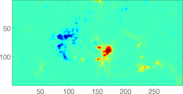
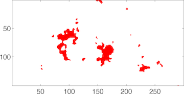
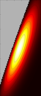
HARP Feature Scale
The following images show how the convolution kernel used for spatial grouping of active regions compares to a small active region at disk center. The units on the top two plots are HMI pixels. The bottom plot shows the convolution kernel at the same scale.
[http://sun.stanford.edu/~turmon/jsoc-wiki/kernel-scale-ar-mag-small.png] [http://sun.stanford.edu/~turmon/jsoc-wiki/kernel-scale-ar-mask-small.png]
[http://sun.stanford.edu/~turmon/jsoc-wiki/ar-grouping-kernel-center-small.png] |
When at the limb, the convolution kernel is foreshortened as shown at right |
[http://sun.stanford.edu/~turmon/jsoc-wiki/ar-grouping-kernel-limb-small.png] |
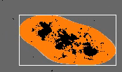
Example
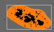
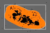
The following images are approximate data segments extracted from the large February 2011 active region. The corresponding HARP contains hundreds of T_REC values; we only show five. The orange blob outlines the contents of the HARP. The black pixels, most of which are inside the HARP, are all pixels declared active in the mask. Some clumps of active pixels are not large enough to constitute a HARP.
The white rectangle is not part of the data segment. It is the bounding box in pixel coordinates which contains the entire HARP, and its coordinates are part of the keywords. There is a corresponding bounding box, not shown, in Stonyhurst latitude-longitude coordinates, which is also recorded in the keywords, as MINLON0, MINLAT0, etc.
[http://sun.stanford.edu/~turmon/jsoc-wiki/track-movie-2011-feb-066-zoom.png] [http://sun.stanford.edu/~turmon/jsoc-wiki/track-movie-2011-feb-126-zoom.png] [http://sun.stanford.edu/~turmon/jsoc-wiki/track-movie-2011-feb-186-zoom.png] [http://sun.stanford.edu/~turmon/jsoc-wiki/track-movie-2011-feb-246-zoom.png] [http://sun.stanford.edu/~turmon/jsoc-wiki/track-movie-2011-feb-306-zoom.png]
Another Example: ImageLink(http://sun.stanford.edu/~todd/jsoc-wiki/Frame.20120509_1000.png,[http://sun.stanford.edu/~todd/jsoc-wiki/Frame.20120509_1000.png,width=250,height=250)]]
Another line: [[http://sun.stanford.edu/~todd/jsoc-wiki/Frame.20120509_1000.png],width=250,height=250]
![http://sun.stanford.edu/~todd/jsoc-wiki/Frame.20120509_1000.png],width=250,height=250](http://sun.stanford.edu/~todd/jsoc-wiki/Frame.20120509_1000.png],width=250,height=250)
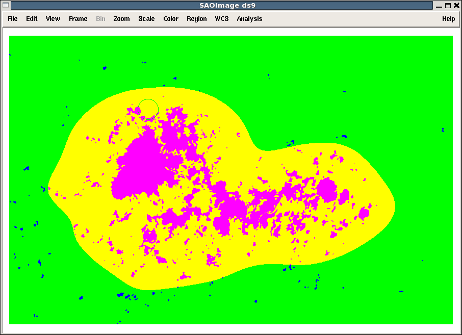
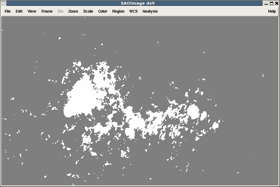
Frame showing HARPs on the Disk on May 9, 2012
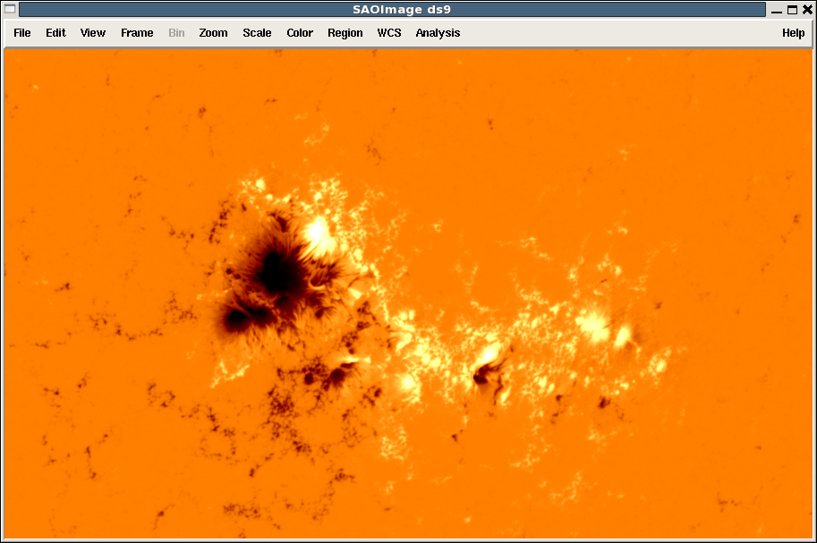
Bitmap for HARP 1638 |
Cut-out of Full Disk Mask |
Cut out of Full Disk Magnetogram |
[http://sun.stanford.edu/~todd/jsoc-wiki/Bitmap1638.20120509_1000.png] |
[http://sun.stanford.edu/~todd/jsoc-wiki/Mask.20120509_1000.png] |
[http://sun.stanford.edu/~todd/jsoc-wiki/Mag.20120509_1000.png] |
Keywords
Besides the standard HMI keywords (observation geometry, time, and WCS), we have these keywords for HARP at each T_REC where it was observed:
Name |
unit |
Description |
MINLON |
degree |
Minimum longitude for disk transit |
MINLAT |
degree |
Minimum latitude for disk transit |
MAXLON |
degree |
Maximum longitude for disk transit |
MAXLAT |
degree |
Maximum latitude for disk transit |
OMEGA |
degree/day |
Rotation rate |
NPIX |
none |
Number of pixels within the identified region |
SIZE |
mH |
Projected area of identified region on image in micro-hemisphere |
AREA |
mH |
De-projected area of identified region on sphere in micro-hemisphere |
NACR |
none |
Number of active pixels |
SIZE_ACR |
mH |
Projected area of active pixels on image in micro-hemisphere |
AREA_ACR |
mH |
De-projected area of active pixels on sphere in micro-hemisphere |
MTOT |
weber |
Sum of absolute LoS flux within the identified region |
MNET |
weber |
Net LoS flux within the identified region |
MPOS_TOT |
weber |
Absolute value of total positive LoS flux |
MNEG_TOT |
weber |
Absolute value of total negative LoS flux |
MMEAN |
gauss |
Mean of LoS flux density |
MSTDEV |
gauss |
Standard deviation of LoS flux density |
MSKEW |
none |
Skewness of LoS flux density |
MKURT |
none |
Kurtosis of LoS flux density |
MINLAT0 |
degree |
Minimum Stonyhurst latitude of pixels within the patch |
MINLON0 |
degree |
Minimum Stonyhurst longitude of pixels within the patch |
MAXLAT0 |
degree |
Maximum Stonyhurst latitude of pixels within the patch |
MAXLON0 |
degree |
Maximum Stonyhurst longitude of pixels within the patch |
FWT_LAT |
degree |
Stonyhurst latitude of flux-weighted center of active pixels |
FWT_LON |
degree |
Stonyhurst longitude of flux-weighted center of active pixels |
FWTPOS_LAT |
degree |
Stonyhurst latitude of flux-weighted center of positive flux |
FWTPOS_LON |
degree |
Stonyhurst longitude of flux-weighted center of positive flux |
FWTNEG_LAT |
degree |
Stonyhurst latitude of flux-weighted center of negative flux |
FWTNEG_LON |
degree |
Stonyhurst longitude of flux-weighted center of negative flux |
T_FRST |
TAI |
T_REC of first frame of this HARPNUM |
T_LAST |
TAI |
T_REC of last frame of this HARPNUM |
Related Data Series
- ["ARmaskDataSeries"]
PatchesFound (obsolete)