hmi.sharp_720s_nrt[606][2012.10.28_18:24:00_TAI].
[1] Parameterizations of the photospheric magnetic field can be correlated with solar activity (Falconer et al., 2002 ; Leka and Barnes, 2003a and 2003b; Schrijver 2007; Mason and Hoeksema, 2010).
[2] It is challenging to collect, store, track, and analyze full-disk vector magnetograms when generally only a small portion of the visible disk, the active regions, produce events.
SHARP stands for Spaceweather HMI Active Region Patch. A SHARP is a DRMS series that contains (1) various spaceweather quantities calculated from the photospheric vector magnetogram data and stored as FITS header keywords, and
(2) 31 data segments (described in detail below),
including each component of the vector magnetic field, the line-of-sight magnetic field, continuum intensity, doppler velocity, error maps and bitmaps.
The data segments are not full-disk; rather, they are partial-disk, automatically-identified active region patches.
SHARPs are calculated every 12 minutes. Often, there is more than one active region on the solar disk at any given time.
Thus, SHARPs are indexed by two prime keys: time, T_REC, and HMI Active Region Patch Number, HARPNUM.
There are four SHARP DRMS series:
[1] hmi.sharp_720s: definitive data with segments in CCD coordinates wherein the vector B has been decomposed into azimuth, inclination, and field,
[2] hmi.sharp_cea_720s: definitive data wherein the vector B has been remapped to a Lambert Cylindrical Equal-Area projection and decomposed into B_radial, B_phi, and B_theta,
[3] hmi.sharp_720s_nrt: near real-time data in CCD coordinates wherein the vector B has been decomposed into azimuth, inclination, and field,
[4] hmi.sharp_cea_720s_nrt: near real-time data wherein the vector B has been remapped to a Lambert Cylindrical Equal-Area projection and decomposed into B_radial, B_phi, and B_theta.
This page describes the methodology for creating SHARPs and uses an example results for NOAA Active Region 11429, which produced an X5.4-class flare on 7 March 2012. The HARPNUM of this region is 1449.
A SHARP numbers can be associated with NOAA AR numbers.
The SHARP data series contain the HMI team's current best effort attempt to determine the vector magnetic field and uncertainties and the data provide a great deal of information. However, the instrument has known limitations due to its spatial and spectral resolution. There are a variety of known and unknown systematic errors and limitations induced by the orbital and other factors. The inversion and disambiguation methods are also known to be far less than perfect. So, please use these data carefully and examine them critically.
See Vector Magnetic Field for more documentation.
Please contact any member of the Vector Field Team with questions or concerns. We welcome your comments and suggestions.
The HMI pipeline analysis code automatically detects
active regions in photospheric line-of-sight magnetograms and
intensity images. This code (i) identifies a patch on the full-disk imagery
that encompasses each active region and (ii) tracks every active
region as it rotates across the face of the solar disk. One active
region crossing the face of the solar disk is referred to as an HMI Active Region
Patch (HARP) and is assigned a HARP number, similar in concept to
a NOAA Active Region number. (We depart from the NOAA Active Region
number because HARPs are detected before NOAA Active Region numbers are
assigned and because we identify many smaller magnetic regions at HARPs.
However, we include the NOAA Active Region number post-facto as FITS
keyword NOAA_AR).
SHARPs use the geometric information in the HARPs to extract the proper
data to perform the calculations for each region at each time step.
There are two kinds of HARPS: (i) near-real time HARPS and (ii) definitive HARPs. Near-real time HARPs are calculated as soon as possible; in this case, the heliographic bounding box for the active region can change from one instant in time to another. Definitive HARPs are defined only after an active region has crossed the face of the disk or 5 days after an active region disappears (whichever comes first); in this case, the heliographic coordinates enclosed by the bounding box for the active region are constant over time. HARPs provide all of the required geometric and heliographic information needed to track active patches in HMI and other solar data sets. Note that HARPNUMs in the nrt and defnitive data series will be different. This is unfortunate, but happens because patches identified in the near real time data sometimes merge with other.
The movie below (courtesy Mike Turmon) shows near-real time HARPs crossing the face of the solar disk in March 2012 (NOAA AR 11429 corresponds to HARP Number 1449):
Definitive HARP data are available at hmi.Mharp_720s; near real time (nrt) HARP data are available at hmi.Mharp_720s_nrt.
The HARP analysis code defines a rectangular (in CCD coordinates)
bounding box, which contains a smooth bounding curve. The bounding box,
which is centered at the flux-weighted centroid, is defined as a HARP;
the area within the bounding curve is defined as an active region. This
information is available within the BITMAP
segment of the SHARP data series.
The HMI Stokes I, Q, U, and V data are inverted within the HARP bounding box by using the Very Fast Inversion of the Stokes Vector (VFISV) code, which assumes a Milne-Eddington model of the solar atmosphere, to yield the vector magnetogram (fill factor assumed unity), Doppler velocity, and other thermodynamic parameters data Borrero et al, 2011). The reported uncertainties are based on the returned variances.
The 180° ambiguity in the transverse component of the image-plane vector
is resolved using a minimum energy method
( Metcalf, 1994;
Leka et al., 2009,
Barnes et al 2012). Input parameters to the disambiguation module
govern the behavior of the global optimization, and differ for the nrt
and definitive data. Pixels below a noise threshold are smoothed after
the optimization (annealing); pixels above the threshold are not.
A spatial mask determines the noise thresholds as a function of solar
radius. (Pixels above this mask threshold can be identified in the
CONF_DISAMBIG segment
of the SHARP series).
Spaceweather quantities (listed in Results[1], below) are calculated
every 12 minuets on the inverted and disambiguated data wherein
the vector B has been remapped to a Lambert Cylindrical Equal-Area
projection and decomposed into Bx, By, and Bz. Some of the spaceweather
quantities are calculated directly on the data.
For quantities that require a computational
derivative, we use a finite-difference method with a 9-point stencil)
and others require a potential field model (such as mean photospheric
excess magnetic energy density). The potential field is calculated
using Green’s functions and a monopole depth of 0.00001 pixels. Only
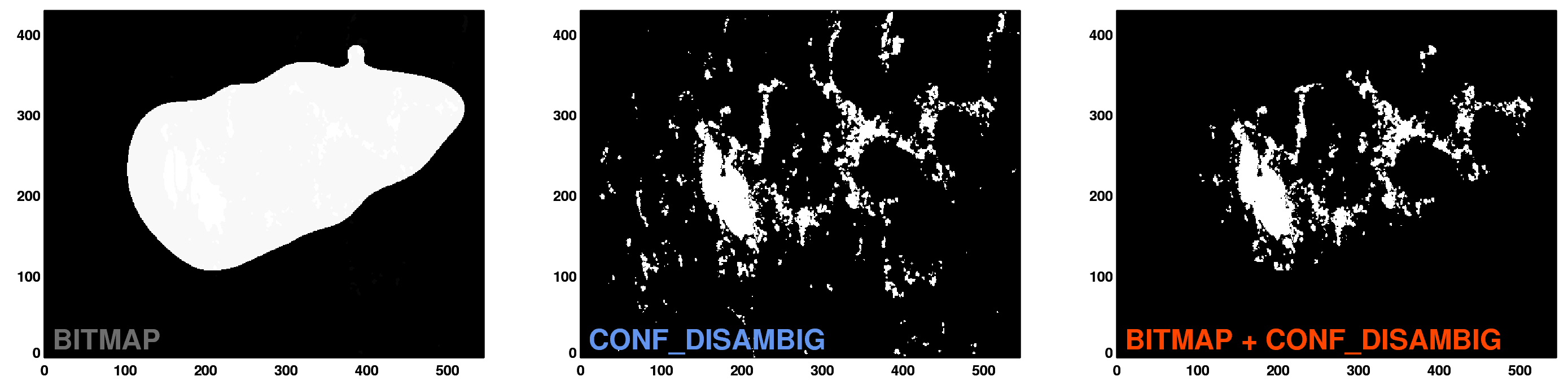
data that are the logical AND of (i) pixels within the smooth
bounding curve in BITMAP and (ii) pixels above the
noise threshold (indicated by the coded values greater than 60 in
CONF_DISAMBIG) contribute to the spaceweather indices.
Below is an example for nrt SHARP 606 at 2012.10.28_18:24:00_TAI; see
hmi.sharp_720s_nrt[606][2012.10.28_18:24:00_TAI].
The SHARP analysis code calculates the following spaceweather quantities for the region (keyword, quantity, units):
USFLUX Total unsigned flux in Maxwells
MEANGAM Mean inclination angle, gamma, in degrees
MEANGBT Mean value of the total field gradient, in Gauss/Mm
MEANGBZ Mean value of the vertical field gradient, in Gauss/Mm
MEANGBH Mean value of the horizontal field gradient, in Gauss/Mm
MEANJZD Mean vertical current density, in mA/m2
TOTUSJZ Total unsigned vertical current, in Amperes
MEANALP Total twist parameter, alpha, in 1/Mm
MEANJZH Mean current helicity in G2/m
TOTUSJH Total unsigned current helicity in G2/m
ABSNJZH Absolute value of the net current helicity in G2/m
SAVNCPP Sum of the Absolute Value of the Net Currents Per Polarity in Amperes
MEANPOT Mean photospheric excess magnetic energy density in ergs per cubic centimeter
TOTPOT Total photospheric magnetic energy density in ergs per cubic centimeter
MEANSHR Mean shear angle (measured using Btotal) in degrees
SHRGT45 Percentage of pixels with a mean shear angle greater than 45 degrees in percent
The SHARP analysis code also calculates the errors in the spaceweather quantities listed above; they are available as follows: (keyword, quantity, units):
ERRVF Total unsigned flux in Maxwells
ERRGAM Mean inclination angle, gamma, in degrees
ERRBT Mean value of the total field gradient, in Gauss/Mm
ERRBZ Mean value of the vertical field gradient, in Gauss/Mm
ERRBH Mean value of the horizontal field gradient, in Gauss/Mm
ERRJZ Mean vertical current density, in mA/m2
ERRUSI Total unsigned vertical current, in Amperes
ERRALP Mean twist parameter, alpha, in 1/Mm
ERRMIH Mean current helicity in G2/m
ERRUSI Total unsigned current helicity in G2/m
ERRTAI Absolute value of the net current helicity in G2/m
ERRJHT Sum of the Absolute Value of the Net Currents Per Polarity in Amperes
ERRMPOT Mean photospheric excess magnetic energy density in ergs per cubic centimeter
ERRTPOT Total photospheric magnetic energy density in ergs per cubic centimeter
ERRMSHA Mean shear angle (measured using Btotal) in degrees
Plots of several quantities computed for HARPNUM 1449 = NOAA AR 11429, appear at the bottom of this web page. One can plot any keyword value directly in JSOC lookdata under the
graph tab.
Data [1]: SHARP Data Segment Descriptions
Below are descriptions for each segment (segment name, units, description) in order of appearance in Lookdata.
The remapped CEA (cylindrical equal area) segments are slightly different (as noted) and only a subset of quantities are present.
MAGNETOGRAM, [Mx/cm2]
The magnetogram segment contains HARP-sized line-of-sight magnetogram data from the DRMS series hmi.M_720s.
CEA version: the field is remapped, but not projected, i.e. it is still the line-of-sight component relative to HMI.
BITMAP, [dimensionless]
The bitmap segment identifies the pixels located within the smooth bounding curve by labeling each pixel with the following:
1 : weak field outside smooth bounding curve
2 : strong field outside smooth bounding curve
33 : weak field inside smooth bounding curve
34 : strong field inside smooth bounding curve
CEA version: same.
DOPPLERGRAM, [m/s]
The dopplergram segment contains HARP-sized dopplergram data from the DRMS series hmi.V_720s.
CEA version: the Doppler velocity is remapped, but not projected, i.e. it is still the line-of-sight component relative to HMI.
CONTINUUM, [DN/s]
The dopplergram segment contains HARP-sized dopplergram data from the DRMS series hmi.Ic_720s.
CEA Version: same.
In order to solve the inverse problem of inferring a vector magnetic field from polarization profiles, the Very Fast Inversion of the Stokes Vector (VFISV) module solves a set of differential equations that fit the following parameters:
INCLINATION, [degrees]
The inclination segment contains the magnetic field inclination with respect to the line-of-sight.
CEA version: not included, See below
AZIMUTH, [degrees]
The azimuth segment contains the magnetic field azimuth. Zero corresponds to the up direction of a column of pixels on HMI’s CCD; values increase counter-clockwise.
CEA version: not included, See below
FIELD, [Mx/cm2]
The field segment contains the
magnetic field strength. Currently, the filling factor is equal to unity,
so this quantity is representative of the magnetic flux density.
It is hard to give a single 'uncertainly' value because of the difference
in noise between the line-of-sight and transverse field components.
Values of 220 Mx/cm2 or less are generally considered to be noise.
CEA version: not included, See below
VLOS_MAG, [cm/s]
The vlos_mag segment contains the velocity of the plasma along the line-of-sight. Positive means redshift. [Note: These data are in cm/s, whereas the dopplergram data are in m/s.]
CEA version: not included
DOP_WIDTH, [mÅ]
The dop_width segment contains the doppler width of the spectral line, computed as if it were assumed to be a Gaussian.
CEA version: not included
ETA_0, [dimensionless]
The eta_0 segment contains the center-to-continuum absorption coefficient.
CEA version: not included
DAMPING, [mÅ]
The damping segment contains the electron dipole oscillation approximated as a simple harmonic oscillator.
In the current version of the code, this parameter is constant and set to 0.5.
CEA version: not included
SRC_CONTINUUM, [DN/s]
The src_continuum segment contains the source function at the base of the photosphere. In the Milne-Eddington approximation, the source function varies linearly with optical depth.
CEA version: not included
SRC_GRAD, [DN/s]
The src_grad segment contains gradient of the source function with optical depth. By definition, src_continuum + src_grad = observed continuum intensity.
CEA version: not included
ALPHA_MAG, [dimensionless]
The segment alpha_mag is defined as the portion of the resolution element that is filled with magnetized plasma. However, in the current version of the code, this parameter is constant and set to unity.
CEA version: not included
CHISQ, [dimensionless]
The segment chisq is a measure of how well the profiles are fit in the least squares iteration. Chisq is not normalized.
CEA version: not included
CONV_FLAG, [dimensionless]
This is currently not calcuated.
CEA version: not included
INFO_MAP, [dimensionless]
The info_map segment identifies the quality index of the inversion output. The higher bits are filled by the inversion module, while the lower ones are updated during the disambiguation step (see below). The index of the higher bits at each pixel is defined as follows:
0x00000000 : Good pixel, with no severe issue.
0x0[0-6]00000 : Same as the convergence index in CONV_FLAG
0x08000000 : Bad pixel, defined as the same criteria as #5 of CONFID_MAP.
0x10000000 : Low Q or U signal. sqrt((Q_0 + ··· + Q_5)^2 + (U_0 + ··· + U_5)^2) was smaller than 0.206 sqrt(I_0 + ··· + I_5 )
0x20000000 : Low V signal; |V_0| + |V_1| + ··· + |V_5| was smaller than 0.206 sqrt(I_0 + ··· + I_5 )
0x40000000 : Low B_los value. |Blos| from magnetogram algorithm was smaller than 6.2 Gauss.
0x80000000 : Missing data
CEA version: not included
CONFID_MAP, [dimensionless]
The confid_map segment identifies the confidence index of the inversion output. The index value at each pixel will take the integer value from 0 (best) to 6(worst), defined as the highest item number satisfying the following conditions:
0: No issue found in the input Stokes
1: Signals for the transverse field component in the input Stokes parameters (Q & U) were weak.
2: Signal for the line-of-sight field component in the input Stokes parameters (V) was weak.
3: Magnetic field signals of both LoS and transverse component were weak.
4: The ME-VFISV iteration did not converge within the iteration maximum.
In the test data release, we set very small , thus, the confidence ε index at most
pixels may be 4.
5: If the difference between the absolute value of the line-of-sight field strength
derived from magnetogram algorithm and the absolute value of the LoS
component from VFISV inversion |B cos(inclination)| is greater than 500
Gauss, we regard the inversion did not well solve the problem.
6: One (or more) of the 24 input Stokes arrays had NaN value.
CEA version: same for nearest un-remapped pixel
The following segments contain formal computed standard deviations
and correlation coeffients derived during the inversion that can be used to determine
the statistical errors of the vector magnetic field.
The standard deviations are the single-parameter lists, the correlation coefficients are the double-parameter entries.
As described in Section 4
of the AR 11158 Vector Magnetic Field, the calculated variances
and covariances are only reliable if the VFISV solution is close to an
absolute minimum.
CEA version: not included
INCLINATION_ERR, [degrees]
AZIMUTH_ERR, [degrees]
FIELD_ERR, [Mx/cm2]
VLOS_ERR, [cm/s]
ALPHA_ERR, [dimensionless]
FIELD_INCLINATION_ERR, [dimensionless]
FIELD_AZ_ERR, [dimensionless]
FIELD_ALPHA_ERR, [dimensionless]
INCLIN_AZIMUTH_ERR, [dimensionless]
FIELD_ALPHA_ERR, [dimensionless]
INCLINATION_ALPHA_ERR, [dimensionless]
AZIMUTH_ALPHA_ERR, [dimensionless]
The following segments are outputs of the disambiguation module:
DISAMBIG, [dimensionless]
The DISAMBIG segment gives more insight into the disambiguation processing.
The SHARP data series always uses the minimum energy method to determine the
reported azimuth and (for CEA) field components. However, two alternative
methods are also computed in weak-field regions and reported in this segment
for consideration by the user. The two other methods are radial-acute and
random. The disambig segment provides the result of the disambiguation
solutions for each pixel by setting the following bits if 180$deg; should
be added to the undisambiguated VFISV azimuth. If multiple bits are
the same, this indicates that the various solutions agree. Currently the
SHARP code uses the minimum energy solution to determine the disambiguation.
bit 1 (lowest bit):
Returned from the minimum energy algorithm. For weak field region pixels
(below the estimated noise mask), additional smoothing is applied (marked
60 in the conf_disambig segment). For the strong field pixels (above the
estimated noise), the minimum energy solution is directly reported (marked
90 in the conf_disambig segment).
bit 2 (middle bit): A random disambiguation solution is adopted for
weak field pixels. The minimum energy solution is adopted for strong field
pixels, i.e. the result will be identical to bit 1.
bit 3 (higher bit): The radial-acute solution is adopted for weak
field pixels. The minimum energy solution is adopted for strong field pixels
(identical to bit 1).
CEA version: not included
CONF_DISAMBIG, [dimensionless]
The conf_disambig segment identifies the final disambiguation solution for each pixel with a value which maps to a confidence level in the result (roughly a probability):
50 : weak field method applied (random/radial/potential)
60 : smoothing applied
90 : annealed
0 : not disambiguated
CEA version: same for nearest un-remapped pixel
INFO_MAP, [dimensionless]
The lower bits of the infomap are updated during this disambiguation step (for higher 4 bits, see the inversion module above). The index of these lower bits is defined as follows:
0x0000 : Not disambiguated.
0x0001 : Weak field, not annealed (only for full disk, filled with potential field, radial acute, or random solution)
0x0003 : Weak field, annealed
0x0007 : Strong field, annealed
The CEA magnetic field values are presented differently, as rectilinear components Br, Btheta, and Bphi at each remapped grid point. Statistical errors are given for each field component, but no cross-correlations are provided. The error in Br, Btheta, and Bphi at each remapped pixel is calculated from the variances of the inverted magnetic field B_total, B_azimuth and B_inclination and the covariances between them. The nearest-neighbor method is used to get the values of the variances and covariances at the original CCD pixel nearest the final remapped pixel. These values are then propagated to derive the errors for Br, Btheta, and Bphi. For further information on vector and map transformations, see: Vector Coordinates and Vector Transformation.
Bp, [Mx/cm2]Bt, [Mx/cm2]Br, [Mx/cm2]Bp_err, [Mx/cm2]Bt_err, [Mx/cm2]Br_err, [Mx/cm2]The following is a log of FITS header keyword CODEVER7 and the changes to the module that create the SHARP data per version of the data.